A Few Notes on the Atomistic Simulations

These programs are classical 2–dimensional molecular dynamics simulations. Such simulations compute the motions of atoms by summing (integrating) all of the forces that the atoms exert on each other. These forces arise from changes in potential energy that depend on the separation distances between the atoms. In principle each atom is interacting with all of the other atoms in the simulation, and thus the forces must be computed between every possible pair of atoms in the simulation. Once the net force is computed for each atom, it's position and velocities are updated and the procedure is repeated.

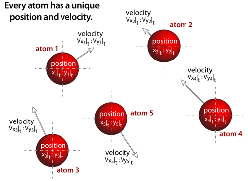
	step 1 Every atom has a unique position and velocity within the simulation, and all of the atomistic properties associated with that specific atom: atomic name, atomic mass, atomic radius, and the interatomic potential functions. All of the atoms are treated as if they are classical particles that move according to Newton's laws of motion (i.e. F=ma; thus, the acceleration (a) acting on any atom is determined by the net interatomic force (F) acting on the the atom divided by the atom's mass (m)).
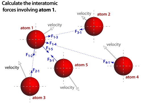
	step 2 The force that acts on an atom depends on the potential surface of the simulation. And ideally, the contributions from every atom in the simulation would be accounted for. Notice that Newton's third law of motion is also invoked, where the forces between each pair of atoms are equal in magnitude but opposite in direction. The forces are derived from the specific interatomic potential functions, which are analytical approximations that depend on the type of bonding being modeled. In these simulations we have modeled van der Waals bonds and ionic bonds.
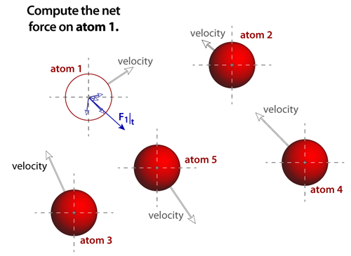
	step 3 The net force acting on any atom is the vector sum of each of the individual forces that arise from the atomic pairs. Some potentials and bonding, such as van der Waals, are short ranged and when pairs of atoms are separated by more than 3 diameters (or so) then the contributions from this pair can be negligible. Other potentials and bonding, such ionic, act over very long distances and neglecting any of their contributions to the forces will create significant problems in the simulation.
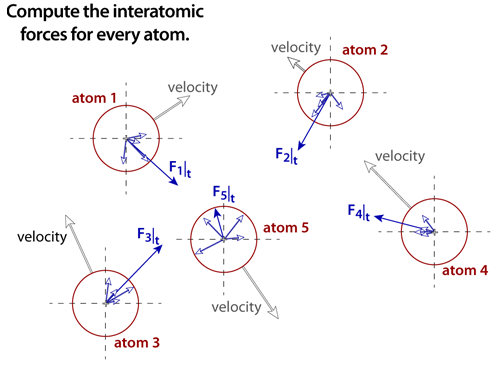
	step 4 The net force must be computed for every atom in the simulation. Assuming that every atomic pair is included in the computation, then the number of computations that must be performed is proportional to the Sum(N), where N is the number of atoms in the simulation (as legend has it, this particular sum was solved by the famous mathematician Karl Friedrich Gauss when he was still a schoolboy: Sum(N) = N(N+1)/2 ). Molecular dynamics simulations require significant computing power because of the extremely large number of computations that must be performed at each time step.
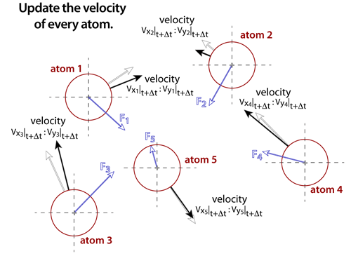
	step 5 Once the net force on each of the atoms is known, the velocities can be estimated from Newton's law assuming that the forces are constant over a small enough increment in time. The time steps in molecular dynamics simulations are very small, typically between femtoseconds (1fs = 1x10-15 s) and picoseconds (1ps = 1x10-12 s). Essentially, the acceleration on the atom is multiplied by the time step to determine the change in velocity. After all of the velocities are determined, a thermostat is used to scale the velocities in such a way that the appropriate energy of the system is maintained.
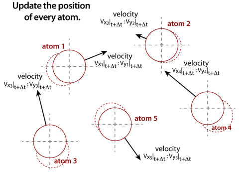
	step 6 The positions of each atom must also be updated. Once the net forces that are acting on the atoms are known, then the positions of each atom can be updated through very accurate integration algoritms. These integrators, such as the Verlet or Leap-Frog algorithms, will increment the position of an atom from its current position based on the net force, velocity, and time step. The integration methods, thermostats, and time steps must be selected based on compromises between accuracy, stability, and speed.
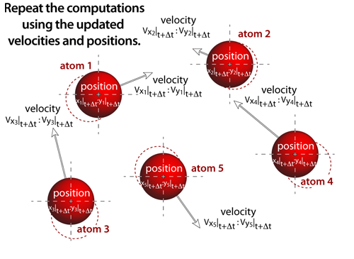
	step 7 Molecular dynamics experiments proceed iteratively, where the output from one iteration becomes the input to the next (i.e. this step now becomes step 1 and the process repeats!). The above sequence of steps represents the computational process that occurs numerous times before the atoms are rendered to the screen. In these simulations, this computational loop will actually be repeated 5-20 times (depending on the number of atoms within the simulation) before the atoms are drawn to the screen. As the number of atoms in the simulation increases the time it takes to compute the new positions and velocities also increases. And in an effort to keep the simulation interactive, the atoms are drawn more frequently as the simulation size increases; this results in the atoms appearing to move more slowly as the number of atoms increases — an unavoidable consequence of complex "real-time" computational simulations.

These simulations also uses "hard" walls as the boundaries. These walls are rigid and inert — when an atom collides with the walls the normal component of its velocity is reversed. Pressure is then calculated in a classical method, by simply keeping track of the momentum changes that occur as a result of wall collisions for fixed intervals in simulation time. When you grab or touch an atom, the motion of your finger defines the velocity of that atom — the temperature will likely fluctuate as you interact with the simulation. When zooming into the simulation the boundaries are dynamically contracting, and any atoms that are caught by the contracting boundary are placed on the edge of the simulation. Eventually, if there is enough space in the simulation, they will work their way back into the simulation space. Finally, and with some apologies, the atoms in these simulations are drawn as polished spheres of specified radii depending on the nature of the simulation.

The Lennard Jones Potential – Atoms In Motion

In the simulation of the noble gas atoms, the van der Waals forces are modeled by the Lennard Jones potential, which is shown graphically below. The simulation temperatures in this module are set to be between 1K and 500K, although you can exceed this by aggressively throwing an atom. The atoms in this simulation are drawn according to their van der Waals radii such that they would just be contacting at the minimum energy separation.

Lennard Jones Potential. The graph above plots the Lennard–Jones potential function, and indicates regions of attraction and repulsion. Atoms try to minimize their potential energy and at the lowest temperatures are sitting at the bottom of the potential curve. When the atomic separations are to the left of the minimum the atoms repel, otherwise they attract one another.

Coulombic Potentials – Salts

This simulation is a mixture of coulombic interactions and van der Waals interactions. For the neutral atom (helium), the van der Waals forces are modeled using the Buckingham potential (U_B). In the Buckingham potential, an exponential function is used to model atomic repulsion (A e ^{(–B R)} ) and the attractive energy follows the classical models of the London dispersion forces (D/R⁶). In this potential function A, B, and D are all constants and R is the separation between the two atoms. In this atomistic simulation, the Buckingham potential is used for all interactions that involve helium. The helium atoms are also drawn according to their van der Waals radius, where the atoms are just touching at the minimum energy location.

 U_B = A e ^{(–B R)} – (D / R ⁶)

The force interaction between ions is based on the Born model, which has 3 distinct contributions to the overall force. Like the Buckingham potential, the repulsive force is exponential. Depending on whether or not the ions have the same or opposite charges, the Coulombic force will be repulsive or attractive, respectively. Finally, there is also the addition of a weak London dispersion force on each of the ions.

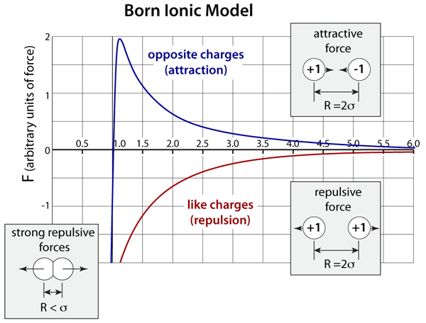
Born Ionic-Model. The graph above plots the Born model for the interatomic forces of a pair of ions; the x–axis is a dimensionless ratio of the separation distance (R) divided the lattice separation distance (σ). This model has an exponential repulsion that is very stiff and it also includes the long-range Coulombic interactions (1/R²) that depend on the product of the ion charge. In this representation positive forces are attractive while negative forces are repulsive.

Simulations with ions are extremely computationally intensive because of the long–range nature of the Coulombic interaction, which follows a 1/R² decay. Because of these long range interactions, the forces and motions of the ions are determined by the integrated contributions from all of the atoms and ions in the simulation. The computations per time step scale by the square of the number of atoms and ions in the simulation (e.g. a simulation with 500 ions is 100 times more computationally intensive then a simulation with 50 ions). A Nose'–Hoover thermostat is also used in this simulation to maintain a nearly constant temperature that is set by the user to be between 1K and 1,500K.

Enjoy the Atoms!